Summary of the work done at Google Summer of Code, 2016, for the OpenDetection Organization

This post is a brief compilation of the details related to the work done as a part of GSoC 2016, for the opensource library OpenDetection. It is a library with a specific focus on the subject of object localization, recognition, and detection in static as well as dynamic sequence of images.

For GSoC, 2016, I was selected to append Convolutional Neural Network related object classification and recognition modules into the library. The Proposal to the library can be accessed at: GSoC Proposal Link.

The following is a brief summary of the work done in the span of three and half months starting from May, 2016,  till Mid-August, 2016.

The modules added to the library are:

• Building the library on CPU as well as GPU Platforms.
• Integration of caffe library.
• Addition of image classification module through c++ version of caffe.
• Addition of CNN training module through c++ version of caffe.
• A customized GTKMM based GUI for creating solver file for training.
• A customized GTKMM based GUI for creating a network file for training/testing.
• A customized GTKMM based GUI for annotating/cropping an image file.
• A Segnet library based image classifier using a python wrapper.
• An Active Appereance model prediction for face images using caffe library.
• Selective Search based object localization algorithm module.

 

Description:

Work1: The primary task undertaken was to make sure that the library compiled on both GPU and non-GPU based platforms. Earlier, the library was restricted to only GPU based platforms, due to the fact that, irrespective of the fact whether cuda library is installed in the system, the library fetched for headers from cuda. With a set of 45 additions and 1 deletions over 7 files, this task was undertaken.

Work2: The next target was to include caffe library components into the opendetection library. Opendetection library is like a pool of object detection elements, and without the integration of Convolutional Neural Networks, it would remain incomplete. there exist a lot of opensource library which support training and classification using CNN, like caffe, keras, torch, theone, etc, of which after we selected caffe, because of its simplicity in usage and availability of blogs, tutorials and high end documentation on the same.

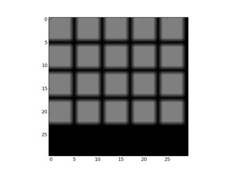
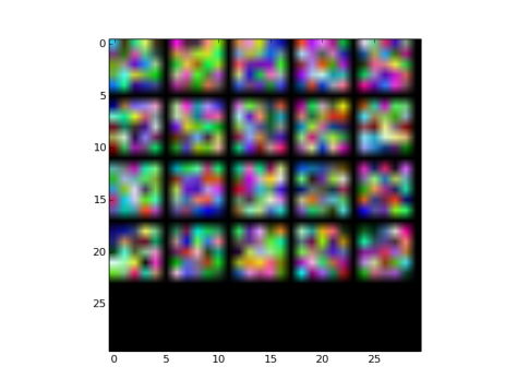
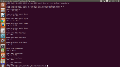
Work3: Once the library was included, the next was to include CNN based image classifier, over a c++ based code. Usually, researchers use the python wrapper provided by the caffe library to train a network or to use trained wieghts and network in classifying an image, i.e., assigning a predicted label to the test image. Herein, the task was completed with around 400 lines of code over 7 files. Any python wrapper reduces the speed of execution and in turn provides a lag in real time based applications. Also, the transfer of memory from cpu to gpu, on gpu based systems, is quite slow when the upper level code is in python. For this reason, we have directly accessed the c++ code files from the library and linked to our opendetection ODDetector class. As an example we have provided the standard Mnist digit classifier. In the example the user just needs to point a network file, trained weights and a test image, and the classification result will be obtained.

Work4: Just adding the classification abilities would make the library only half complete. Hence, for this reason we added the module which would enable the users to train their own module. With a total of around 250 changes made to 5 files, this training class was added to ODTrainer. User would only need to point towards the network and the solver file. Here again, a training example is added using Mnist digit dataset.

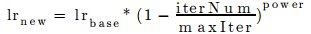
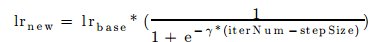
Work5: As stated above, a cnn based training requires a network file and a solver file. Any solver in caffe library has around 20 parameters. It is a tedious job to write the solver file from scratch, everytime a training has to be commenced. For this reason, to facilitate user feasibility over the solver properties a GUI has been introduced. This GUI has all the parameters involved in solver file. Also the user while using the gui has the facility to include or exclude a parameter. This particular commit had changes added or additions made to 9 files. The most crucial one was to add gtkmm library files to the source. GTKMM, link to understand gtkmm, is a library for involvement of gui based applications. We decided to move with GUI inclusion because, to make user handle solver file in an effective way, a set of 19 parameters had to be handled. If it were upto the c++ arguments to facilitate these 19 parameters, the outcome would have been a very cumbersome application. Also, not all parameters were to be added to the solver always, so a GUI appeared to be the most feasible option from the user’s end. A set of around 1250 lines of code made this module integrated into the opendetection library. The following are a few features of the GUI:

• The above code promts the user if any mistake is made from user-end.
• Pressing update button every time may be time consuming, hence the latest commits involve the fact that without pressing the buttons the parameters cab ne edited
• The main function of the update buttons after every parameter is make sure that, for future developments, if the intermediate parameters are to be accessed, the current version enables it.
• Not many open source libraries had this functionality

Work6: After solver, the next important thing to training is network file. A network file in CNN has the structure of the CNN, the layers, their individual properties, weight initializers, etc. Like the solver maker, we have created a module which provides a GUI to make this network. Every network has lot many properties, writing them manually into the file is a time consuming process. For this reason, the GUI was implemented, so that with just a few clicks and details any layer could be added to the network. a) The activation category includes the following activation layers

• Absolute Value (AbsVal) Layer
• Exponential (Exp) Layer
• Log Layer
• Power Layer
• Parameterized rectified linear unit (PReLU) Layer
• Rectified linear unit (ReLU) Layer
• Sigmoid Layer
• Hyperbolic tangent (TanH) Layer

b) The critical category includes the most crucial layers

• Accuracy Layer
• Convolution Layer
• Deconvolution layer
• Dropout Layer
• InnerProduct (Fully Connected) Layer
• Pooling Layer
• Softmax classification Layer

c) The weight initializers include the following options

• Constant
• Uniform
• Gaussian
• Positive Unit Ball
• Xavier
• MSRA
• Bilinear

d) Normalization layer includes the following options

• Batch Normalization (BatchNorm) Layer
• Local Response Normalization (LRN) Layer
• Multivariate Response Normalization (MVN) Layer

e) Loss Layer includes the followin optons: -Hinge Loss Layer

• Contrastive Loss Layer
• Eucledean Loss Layer
• Multinomial Logistig Loss Layer
• Sigmoid Cross Entropy Loss Layer

f) Data and Extra Layers:

• Maximum Argument (ArgMAx) Layer
• Binomial Normal Log Likelihood (BNLL) Layer
• Element wise operation (Eltwise) Layer
• Image Data Layer
• LMDB/LEVELDB Data Layer

g) Every Layer has all the parameters listed in the GUI, of which the non compulsory parameters can be kept commented using the radiobutton in the GUI,

h) One more important feature included is that user can display the layers. The facility to delete any particular layer, or add any layer in the end or in between two already implemented layers is also feasible through the usage of the GUI.

These properties of the GUI were made possible with a set of aorund 6500 lines of code over a range of arounf 12-15 files.

Work7: Active Appereance Model feature points over the face have had many application like emotion detection, face recognition etc. It’s of the personal researches we have undertaken which is based on finding these feature points using Convolutional Neural Networks. The network and the trained weights presented in the example in the library is one of the base models we have used. The main reason to add this feature was to show as to how widespread the uses of the integration of caffe library with opendetection could be to the users. Very few works exist on this end, and hence the purpose behind taking up the research. This is a very crude and preliminary model of the research, just for the young users to be encouraged as to the extent to which cnn may work and how opendetection algorithm would help facilitate the same.

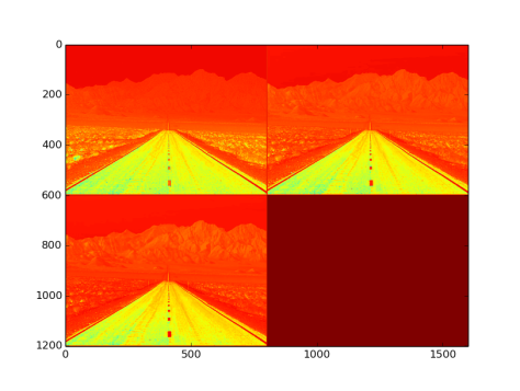
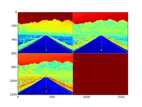
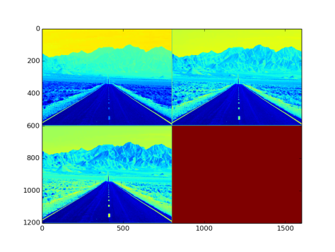
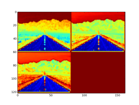
Work8: Object reconition has two components: object localization and then classification. Classification module has already be included in the system, the localization part is introduced in this work. The task of object localization has been completed using selective search algorithm. The algo, when put simply, involves, Graph based image segmentation, followed by finding different features of the all the segmented parts, then finding closeness between the features of the neighboring parts and finally merging the closest parts and continuing futher till the algorithm is breaked. The image segmentation was adopted from Graph based image segementation mentioned here with proper permissions. The next part involved image preprocessing, which had conversion of BGR image to YCrCb, equalizing the first channel and reconversion of equalized YCrCb image to BGR color type. This was followed by the steps: image is stored in “.ppm” format as the segmentation code only prefers image in that format. Image is then segmented using the segment_image function and to find the number of segments, num, it is converted to grayscale and the number of colors there then represent the number of segments. The next step is to create a list of those segments. It is not often possible to create an uchar grayscale image mask with opencv here, because, opencv supports color version from 0 to 255 and in most cases the segments are greater than 255. Thus, we first store, every pixel’s value in the previous rgb image with the pixel’s location into a text file named “segmented.txt”.Finally, the steps were adopted, calculating histogram of the different features ( hessian matrix, orientation matrix, color matrix, differential excitation matrix), finding neighbors for each of the clustered region, finding similarities( or closure distance) between two regions based on the histogram of different features, merging the closest regions removing very small and very big clusters, and adding ROIs to images based on merged regions. This selective search has a set of 13 parameters which drive the entire algo here. The work here was completed with addition of around 2000 lines of code.

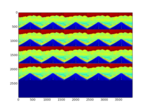
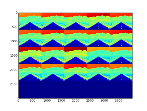
Work9: Segnet is a caffe derived library used for object recognition and segmentation purposes. It is a widely used library and the components are very much similar to caffe library. Thus there existed this logical compulsion to include the library so that the users may use segnet based training/classification/segmentation examples through opendetection wrapper. Addition of this library would allow segnet library users to attach it to opendetection in way as done with caffe library. Herein, the example included for now, is a python wrapper based image segmentation preview. The network and the weights are adopted from segnet example module.

Work10: Any image classifier training requires the dataset to be annotated. For this reason, we have added an annotation tool, which will enable users to label, crop or create bounding boxes over an object in image. The output of this tool is customized in a way which is required by the caffe library.

The features and some usage points involved are:

• User may load a single image from a location using the “Select the image location” button or the user may point towards a complete image dataset folder.
• Even if the user points to a dataset folder, there exists an option of choosing an image from some another location while the annotation process is still on.
• Even if user selects a single image, the user may load more single images without changing the type of annotation.
• The first type of annotation facility is, annotating one bounding box per image.
• The second, annotating and cropping one bounding box per image.
• The third one, annotating multiple bounding boxes per image, with attached labels.
• The fourth one, cropping multiple sections from same image, with attached labels.
• The fifth one, annotationg a non rectangular ROI, with attached labels.
• If a user makes mistake in annotation, the annotation can be reset too.

Note: Every image that is loaded, is resized to 640×480 dimensions, but the output file has points of the bounding boxes as the original image size

The output files generated in the cases have annotation details as,

• First case, every line in the output text file has a image name followed by four points x1 y2 x2 y2, first two representing top left coordinate of the box and the last two representing bottom right coordinates of the box.
• Second case, every line in the output text file has a image name followed by four points x1 y2 x2 y2, first two representing top left coordinate of the box and the last two representing bottom right coordinates of the box. The cropped images are stored in the same folder as the original image, with name, <original_image_name>_cropped.<extension_of_the_original_image>
• Third case, every line in the output text file has a image name followed by a lebel and then the four points x1 y2 x2 y2, first two representing top left coordinate of the box and the last two representing bottom right coordinates of the box. If there are multiple bounding boxes, then after image name there is a label, then four points, followed another label, and the corresponding four points and so on.
• Fourth case, Once the file is saved, the cropped images will be saved in the same forlder as the original image with name as <original_image_name>_cropped_<label>_<unique_serial_id>.<extension_of_the_original_image>.
• Fifth case, The output of the file will be saved as filename, followed by an unique id to the ROI, label of the roi, set of points in the roi, then again another id, its label and the points and so on.

To select any of these cases, select the image/dataset and then press the “Load the image” button.

First case usage

• Select the image or the dataset folder.
• Press the “Load the image” button.
• To create any roi, first left click on top left point of the supposed roi and then right click on the bottom right point of the supposed roi. A green rectangular box will appear.
• Now, if its not the one you meant it, please click “Reset Markings” Button and repoint the new roi.
• If the ROI is fine, press “Select the ROI” button.
• Now, load another image or save the file.

Second case usage

• Select the image or the dataset folder.
• Press the “Load the image” button.
• To create any roi, first left click on top left point of the supposed roi and then right click on the bottom right point of the supposed roi. A green rectangular box will appear.
• Now, if its not the one you meant it, please click “Reset Markings” Button and repoint the new roi.
• If the ROI is fine, press “Select the ROI” button.
• Now, load another image or save the file.

Third case usage

• Select the image or the dataset folder.
• Press the “Load the image” button.
• To create any roi, first left click on top left point of the supposed roi and then right click on the bottom right point of the supposed roi. A green rectangular box will appear.
• Now, if its not the one you meant it, please click “Reset Markings” Button and repoint the new roi.
• If the ROI is fine, please type an integer label in the text box and press “Select the ROI” button.
• Now, you may draw another roi, or load another image, save the file.
• Note: In the third case, the one with multiple ROIs per image, if a boundix box is selected for an image and you are trying to make another and press the reset button, the selected roi will not be deleted. Any selected roi cannot be deleted as of now.

Fourth case usage

• Select the image or the dataset folder.
• Press the “Load the image” button.
• To create any roi, first left click on top left point of the supposed roi and then right click on the bottom right point of the supposed roi. A green rectangular box will appear.
• Now, if its not the one you meant it, please click “Reset Markings” Button and repoint the new roi.
• If the ROI is fine, please type an integer label in the text box and press “Select the ROI” button.
• Now, you may draw another roi, or load another image, save the file.
• Once the file is saved, the cropped images will be saved in the same forlder as the original image with name as <original_image_name>_cropped_<label>_<unique_serial_id>.<extension_of_the_original_image>

Fifth case usage

• Select the image or the dataset folder.
• Press the “Load the image” button.
• To create any roi, Click on the points needed only with left click.
• Now, if its not the one you meant it, please click “Reset Markings” Button and repoint the new roi.
• If the ROI is fine, please type an integer label in the text box and press “Select the ROI” button. A gree color marking covering the region and passing through the points you have selected will appear.
• Now, you may draw another roi, or load another image, save the file.

Thus, this tool, is an extremely important addition to the project and was added as a set of 1600 lines of code on around 6-8 files in the opendetection library.

The corresponding source-codes, brief tutorials and commits, can be accessed here

For Compilation of the library, refer to the link here

Upcoming Work:

a) Resolve the issue of cpp version of AAM and segnet based classifier

b) Heat map generator using cnn ( will require time as its is quite research intensive part)

c) Work to be integrated with Giacomo’s work and to be pushed to master.

d) API Documentation for the codes added.

e) Adding video Tutorials to the blog.

 

Happy Coding 🙂 !!!

ANN: Chapter 3. Deep Learning using caffe-python

Convolutional Neural Networks, abbreviated as CNN, is an integral part of computer vision and robotics industry. To first understand what a neural network is please refer: Link1 & Link 2 . A huge research is being done in the fields of vehicle detection convolutional neural networks. This post is mainly focused over caffe’s(python) implementation of CNN networks: Link 3 . This research over understanding the caffe library is done for my ongoing undergraduate thesis. Hoping that you already have installed caffe and know the basics of CNN. Let’s start it then 🙂

A Convolutional neural networks is defined with the broad combination of:

1. Data structure, type, and format.
2. Layers, their properties and the arrangement in space.
3. Weight initializers at the beginning of the training.
4. Loss function to help the back-propagation.
5. Training optimizers and solvers like Stochastic gradient descent algorithm, etc. Structure training parameters like learning rate, decay rate, number of iterations, batch size, etc.
6. Computational Platform

Note:

• All the points highlighted using color represent a variable that effects training.
• All the points highlighted using color represent a file.

• Every file/image/code is available at: [ Github Repository ]

• Every code begins with setting up root directory to caffe, please make certain changes according to your installations.

1. Data:

In caffe implementation, this is considered a layers, actual data is called as blob. Any structure in caffe is implemented using a protobuffer file with extension as “.prototxt”. It is a fairly easier way of representing any structure when compared the same implementation in a XML file. This layer(Data) [Caffe Data Layer] mainly takes inputs from these specific types of file formats, HDF5, LMDB, LEVELDB, Image.

1.1 Type: Image

• The first step is to create/obtain a dataset and labeled dataset. The parent folder (current working directory) must have a folder containing the dataset and two text files, say, Train.txt and Test.txt which would contain the path of each of the images. Note the Test here means validation set. We would in this blog consider Mnist Dataset and LeNet network[ LeNet].
• Get the CSV format from here: [Mnist Dataset in CSV Mode] . The file to convert these CSV files to PNG for mat is read_file_train.cpp . This file expects the file structure as
  • Parent Folder
    • Dataset
      • Train
      • Test
        
    • read_file_train.cpp

Note: This file uses OpenCV libraries.

• Here the variable to be considered are
  • Number of training images ( Here 60,000)
  • Number of training images which are used for validation ( Here 5000)
  • Size of the training images ( here its 28×28)
• Note: There are basically three such “.prototxt” files
  • train_test.prototxt ( you may name these anything) : Contains training network structure.
  • deploy.prototxt : Contains testing network structure.
  • Solver: Contains training parameters.
• Now the description is translated into “.prototxt” file. For Train_set: imageDataLayer_example.prototxt.
  • Any layer is initiated with “layer{}”. [ Data Layer Caffe]
  • “name:” represents its unique identity so that the structure can be implemented.
  • “top”, “bottom”, represent what is next it, and behind it, respectively. It’s a bottom-up structure. The lowest layer is always the Data Layer.
  • This layer has two things on “top” of it, namely the “data” blob and the “label” blob.
  • “phase” determines the part of training, train/validation, which will use the data provided.
  • “transform_param”, is from a class dataTransformer [ Data Transformer]. It does scaling of input, subtracting mean image from entire dataset, to make the dataset zero-centric. The mean parameter is described as mean_file: “mean.binaryproto”.
• Creating mean.binaryproto file:
  • There may be many ways to do it, and here’s one of them.
  • In the caffe_root_directory there will be two exe files, ./ convert_imageset and ./compute_image_mean.
  • Copy these files into your Parent Directory.
  • Now Run “chmod +x convert_imageset” in the terminal
  • Then “chmod +x compute_image_mean”, to make them executable
  • First we will convert images to lmdb format, then calculate mean and store in mean.binaryproto
  • ‘./convert_imageset “” Train.txt Train’. LMDB formatted Dataset is stored in Train folder
  • ‘./compute_image_mean Train mean.binaryproto’
  • Repeat the same for Test.txt, if you need the mean there too.
•  The “scale” parameter normalizes every pixel, by dividing it by 256, i.e., 1/256 = 0.00390625
• “source” stores the filename of the annotated text file, “Train.txt”, it has format
  • path_to_image/image_name.extension label
• A stochastic approach of training, rather modifying the weights to be specific, doesn’t depend on the entire dataset in each training, it uses a set of images randomly selected in batches for every iteration. This batch size is given by “batch”
• “new_height” & “new_width” are resizing parameters
• “crop_size” crops the image with given square dimensions but from random portions and uses fro training.
• Similarly for Test Phase.

1.2 Type: LMDB

• A lmdb [LMDB]type dataset can be created using ./convert_imageset as stated above( See 1.1, at the part of creating mean.binaryproto file)
• Now the description is translated into “.prototxt” file. For Train_set: lmdbDataLayer_example.prototxt
• Most of the things remain same, except
  • type: “data”
  • In the “data_param”, it is mentioned “backend: lmdb”
• Similarly for Test Phase

1.3 Type: LEVELDB

• A leveldb [ Data Layer] [ LEVELDB ] type dataset can be created using ./convert_imageset as stated above( See 1.1, at the part of creating mean.binaryproto file) with a slight exception “ ./convert_imageset “” Train.txt leveldb -backend leveldb”
  • ./convert_imageset [ ] has these parameters :
    • -backend (The backend {lmdb, leveldb} for storing the result) type: string default: “lmdb”
    • -check_size (When this option is on, check that all the datum have the same size) type: bool default: false
    • -encode_type (Optional: What type should we encode the image as (‘png’,’jpg’,…).) type: string default: “”
    • -encoded (When this option is on, the encoded image will be save in datum) type: bool default: false
    • -gray (When this option is on, treat images as grayscale ones) type: bool default: false
    • -resize_height (Height images are resized to) type: int32 default: 0
    • -resize_width (Width images are resized to) type: int32 default: 0
    • -shuffle (Randomly shuffle the order of images and their labels) type: bool default: false
• Now the description is translated into “.prototxt” file. For Train_set: leveldbDataLayer_example.prototxt
• Most of the things remain same, except
  • type: “data”
  • In the “data_param”, it is mentioned “backend: leveldb”
• Similarly for Test Phase

1.4 Type: HDF5 (implementation in training not tested by me here)

• What is hdf5 format?: [ HDF5]
• Note: This can create an array for labels too, but here for mnist we dont require it
• Convert image dataset to hdf5
  • Dataset Folder
  • Train.txt
  • Run in terminal: ipython convertImage2hdf5.py
    • It will create a train.h5 file. It can be opened using HDF tools
• see “hdf5DataLayer_example.prototxt”
  • source: “hdf5Ptr.txt”
    • It contains the path to train.h5 .

 

2. Layers:

A LeNet structure as limited number of layers, unlike that, this section provides a brief description(implementation details) of all the kinds of layers that can be constructed with caffe library. The example prototxt files are of format used in testing layers, its just that the DataLayer is not included and input data dimensions are given by “input_dim: int_value”. This parameter is called 4 times, first for batch_size(N), second for image_channel_size(C), third for image_height(H), and finally for image_width(W), i.e., the blob is a 4-D array of format NxCxHxW. The width is leftmost index in the array, i.e., arr[][][][], the last [] changes the index of width. Also in most of the cases in here, the file understandLayers.py (sufficiently commented) [ Classification Example Caffe]file is used to demonstrate the how an image is effected by the layers.

Note: In the demonstration, weight initializers will be default, their effect will be understood in next section. 

The image under observation is:

Fig 1: Input Image to study layers

2.1 Absolute Value Layer

• See “absValLayer_example.prototxt”.
• The type is “absVal”. • Function: y = m o d (x ), where, m o d ( ), represents modulus function.
• Input to the layer: NxCxHxW sized blob
• Output from the layer: NxCxHxW sized blob. Fig 2. is an image with three channel outputs after passing from this layer

Fig 2: 3 channel output after being passed through absVal layer

2.2 Accuracy Layer

• see “accuracyLayer_example.prototxt”.
• type : “Accuracy”
• Usage: After the final layer. It is used in the TEST phase.
• Takes input as the final layers output and the labels.
• Used for calculating the accuracy of the training during TEST phases.

2.3 ArgMax Layer

• see “argMaxLayer_example.prototxt”
• type: “ArgMax”
• Calculates index of k maximum values across all dimensions
• Usage: After classification layer to get the top-k predictions
• Parameters:
  • top_k: sets the value of k
  • out_max_val: true/false ( if true returns pair (max_index, max_value) the input)
• Fig3. Shows how the output looks, (doesn’t makes sense to get a figure out of the max_values, but still)

Fig 3: Output after being passed through argMax layer

2.4 Batch Normalization layer

• see “batchNormLayer_example.prototxt”
• Normalizes the input data to achieve mean = 0 and variance = 1.
• Input to the layer: NxCxHxW sized blob
• Output from the layer: NxCxHxW sized blob. Fig 4. is an image with three channel outputs after passing from this layer

Fig 4: Output after batch normalization

2. 5 Batch Reindex layer

• type: BatchReindex
• To select, reorder, replicate batches

2.6 BNLL Layer

• see “bnllLayer_example.prototxt”
• type: “BNLL”
• bnll: Binomial normal log likelihood [ BNLL ] • Function: y = x + lo g (1 + e x p ( – x )) , if x>0

y = l o g (1 + e x p (x )); if x<=0

• Input to the layer: NxCxHxW sized blob
• Output from the layer: NxCxHxW sized blob. Fig 5. is an image with three channel outputs after passing from this layer

Fig 5: Output after passing through bnll layer

2.7 Concat Layer

• type: “Concat”
• Used to concatenate set of blobs to one blob
• Input: K inputs of dimensions NxCxHxW
• Output: if parameter:
  • axis = 0: Dimension : (K*N)xCxHxW
  • axis = 1: Dimension : Nx(K*C)xHxW

2.8 Convolution Layer

• The most important layer
• see “convLayer_example.prototxt”
• param{} : Its for learning rate and decay rate for filters and biases. First call is for learning rate, next call is for biases. That is why it is written two times.
  • lr_mult: For learning rate
  • decay_mult: Decay rate for the layer Note: This is common to many layers
• type: “Convolution”
• Parameters:
  • num_output(N) : number of filters to be used
  • kernel_size(F): Size of the filter. This can also be mentioned as:
    • kernel_w(F_W)
    • kernel_h(F_H)
  • stride(S): Decides by how much pixel should the filter move over a particular blob in blob dimensions. This is the main reason for sparsity in CNNs. This can also be mentioned as:
    • stride_w(S_W)
    • stride_h(S_H)
  • pad(P): Mentions the size of ZERO padding to be put outside the boundary of the blob. This can also be mentioned as:
    • pad_w(P_W)
    • pad_h(P_H)
  • dilation: Default->1. For morphological operations
  • group: see [ http://colah.github.io/posts/2014-12-Groups-Convolution/%5D
  • bias_term: For adding biases
  • weight_filler: Will be discussed in later sections
  • Input: Blob size of NxCxHxW
  • Output Blob size of N’xC’xH’xW’
    • N’ = N
    • C’ = K
    • W’ = ((W  – F_W + 2 * (P_W ))/S_W ) + 1
    • H’  = ((H  – F_H + 2 * (P_H ))/ S_H ) + 1
  • Fig 6 shows the filters initialized with guassian distribution, and Fig 7 shows the convoluted outputs. ( Note: The actual dimensions of filters/blobs are modified to fit in as images)

Fig6: Filters initialzed for convolutional layer

Fig 7: Output blob as images after being passed through convolution layers

2.9 Deconvolution Layer

• see “deconvLayer_example.prototxt”
• Everything same as convolutional layer but, the forward and backward functionalities are reversed.
• Even the parameter functioning is reversed, i.e., pad removes padding, stride causes upsampling, etc.
• Fig 8 shows deconvoluted image blob formed from Fig.7 convoluted images. Exact input image is not restored here because of random weight initialization

Fig 8: Output after passing through deconvolution layer

Note: This layer can have mutilple channeled output too.

2.10 Dropout Layer

• Note: Works only in TRAIN phase
• see “ dropoutLayer_example.prototxt”
• Function: Sets a portion of pixels to 0, other wise works as absVal Layer.
• Parameters:
  • dropout_ratio: Probability that the current pixel value will be set to zero
• Helps in decreasing the training time.
• Input to the layer: NxCxHxW sized blob
• Output from the layer: NxCxHxW sized blob. Fig 9. is an image with three channel outputs after passing from this layer

Fig 9: Output after dropout layer

2.11 Element Wise Layer

• type: Eltwise
• For Element wise summation on one or multiple same sized blobs.
• see “eltwiseLayer_example.prototxt”
• Sums up every pixel, basically adds two blobs
• Input to the layer: NxCxHxW sized blob
• Output from the layer: NxCxHxW sized blob. Fig 10. is an image with three channel outputs after passing from this layer

Fig 10: Output after passing through eltwize Layer.

2.12 Embed Layer

• type: Embed
• Same as a fully connected layer, see 2.17
• Except the output blob is a 1D 1-hot vectors. 1-hot vectors are those vectors which have only one element which has value greater than 0, rest all will be zero. [ One Hot Vector ]

2.13 Exponential Layer

• see “expLayer_example.prototxt”
• type: Exp
• Function: y = γ^(α*x + β)
• Parameters:
  • Base (γ) : default: e
  • Scale (α) : default: 1
  • Shift (β) : default: 0
• Input to the layer: NxCxHxW sized blob
• Output from the layer: NxCxHxW sized blob. Fig 11. is an image with three channel outputs after passing from this layer

Fig 11: Output from exponential layer with default parameters

2.14 Filter Layer

• type: Filter
• Takes more than one blobs. The last blob is the filter_decision blob. This blob must be a singleton. The selector blob must be of dimensions Nx1x1x1. So whichever element in this blob is 0, the corresponding indexed batch will become 0, and the other ones will be passed as it is.

2.15 Flatten Layer

• type: Flatten
• Takes a blob and flattens its dimensions
• Input dimension: NxCxHxW
• Output dimension: Nx(C*H*W)x1x1

2.16 Image to Col Layer

• type: Im2col
• Used by convolution layer to convert 2D image to a column vector

2.17 Inner Product Layer

• In common terms called as Fully Connected layer
• The next most important layer after convolution layer • see “innerProductLayer.prototxt”
• type: InnerProduct
• Parameter:
  • num_output: Number of neurons in the output layer
  • weight, bias, layer param are same as in convolution layer

2.18 Log Layer

• see “logLayer_example.prototxt”
• type: Log
• Function: 
• Parameters:
  • Base (γ) : default: e
  • Scale (α) : default: 1
  • Shift (β) : default: 0
• Input to the layer: NxCxHxW sized blob
• Output from the layer: NxCxHxW sized blob. Fig 12. is an image with three channel outputs after passing from this layer

Fig 12: Output from logLayer with default parameters

2.19 LRN Layer

• see “lrnLayer_example.prototxt”
• type: LRN
• LRN: Local response Normalization [ LRN Layer ] [ LRN Function ]
• Parameters
  • local_size: The size of local kernel. Must be an odd number
  • alpha: ideally 0.0001
  • beta: ideally 0.75
  • k: ideally 2
  • norm_region: WITHIN_CHANNEL or ACROSS_CHANNELS (self explanatory)
• Input to the layer: NxCxHxW sized blob
• Output from the layer: NxCxHxW sized blob. Fig 13. is an image with three channel outputs after passing from this layer

Fig 13: Output from lrnLayer with default parameters

2.20 MVN Layer

• See “mvnLayer_example.prototxt”
• type: MVN • MVN: Multi Variate Normalization [ MVN Distribution]
• Parameters:
  • across_channes: bool type
  • normalize_variance: bool type
  • eps: Scalar shift (see link above)
• Input to the layer: NxCxHxW sized blob
• Output from the layer: NxCxHxW sized blob. Fig 14. is an image with three channel outputs after passing from this layer

Fig 14: Output after MVN layer

2.21 Pooling Layer

• This is again one of the most frequently used layers in a CNN
• see “poolingLayer_example.prototxt”
• type: Pooling
• Parameters:
  • kernel_size: same as in convolution layer
  • stride: same as in convolution layer
  • pad: same as in convolution layer
  • pool:
    • MAX: Takes max element of the kernel
    • AVE: Takes average of the kernel
    • STOCHASTIC: Not implemented
• Input Dimensions: NxCxHxW
• Output Dimensions: N’xC’xH’xW’ (see 2.8)
  • N’ = N
  • C’ = C
  • W’ = ((W – F_W + 2 * (P_W ))= S_W ) + 1
  • H’  = ((H – F_H + 2 * (P_H ))= S_H ) + 1
• Fig 15. is an image with three channel outputs after passing from this layer

Fig 15: Pooling layer applied with F = 10 and S = 10

2.22 Power Layer

• see “powerLayer_example.prototxt”
• type: Power
• Function: 
• Parameters:
  • Power (γ) : default: 1
  • Scale (α) : default: 1
  • Shift (β) : default: 0
• Input to the layer: NxCxHxW sized blob
• Output from the layer: NxCxHxW sized blob. Fig 16. is an image with three channel outputs after passing from this layer

Fig 16: Output after passing through power layer with power = 2, scale = 1, and shift = 2

2.23: PReLU Layer

• The rectified activation function most commonly used as it does not saturate like sigmoid and is even faster. This is prefered over simple ReLU for the fact that it considers the negative input also. [ https://en.wikipedia.org/wiki/Rectifier_ (neural_networks) ]
• see “preluLayer_example.prototxt”
• type: PReLU
• Function: y = m a x ( 0, x ) + α * m in (0, x ), the slope parameter α is constant
• Parameters:
  • channel_shared: bool type (Same alpha for all the channels)
  • filler(will be discussed in later sections)
• Input to the layer: NxCxHxW sized blob
• Output from the layer: NxCxHxW sized blob. Fig 17. is an image with three channel outputs after passing from this layer

Fig 17: Output after PReLU layer with channels shared and gaussian type filler

2.24 ReLU Layer

• Rectified Linear Units
• PReLU with slope parameter α as non-constant, as in specified by user
• see “reluLayer_example.prototxt”
• type: ReLU
• function: y = m a x ( 0 , x ) + α * m in (0 , x )
• Parameters:
  • negative_slope: Default: 0
• Input to the layer: NxCxHxW sized blob
• Output from the layer: NxCxHxW sized blob. Fig 18. is an image with three channel outputs after passing from this layer .

Fig 18: Output after ReLU layer with a negative image input

2.25 Sigmoid Layer

• see “sigmoidLayer_example.prototxt”
• type: Sigmoid
• Used as an activation function
• Function : 
• Input to the layer: NxCxHxW sized blob
• Output from the layer: NxCxHxW sized blob. Fig 19. is an image with three channel outputs after passing from this layer

Fig 19: Output after Sigmoid Layer

2.26 Softmax Layer

• see “softmaxLayer_example.prototxt”
• type: Softmax
• Function: [ source: Softmax Layer ]
• Parameters:
  • axis: the central axis (integer type)
• Input to the layer: NxCxHxW sized blob
• Output from the layer: NxCxHxW sized blob. Fig 20. is an image with three channel outputs after passing from this layer

Fig 20: Output after Softmax Layer

2.27 Split Layer

• type: Split
• Creates multiple copies of the input to be fed into different layers ahead simultaneously

2.28 Spatial Pyramid Pooling : Will Update this soon

2.29 TanH Layer

• see “tanhLayer_example.prototxt”
• type: TanH
• Function : 
• Input to the layer: NxCxHxW sized blob
• Output from the layer: NxCxHxW sized blob. Fig 21. is an image with three channel outputs after passing from this layer

Fig 21: Output after passing tanH layer

 

3. Weight Initializers

They are important because of the fact that initializing weights at complete random may lead to early saturation of the weights. In the examples below, layer used is convolutional layer.

3.1 Constant Filler

• See “constantFiller_example.prototxt”
• type: constant
• Fills the weights with a particular constant, default value is 0
• Parameters
  • value: double type
• Fig 22 and Fig 23 show the filters and effects respectively

Fig 22: Constant fillers of value 0.5

Fig 23: Effect on image by constant type filler and convolutional layer

3.2 Uniform Layer

• see “uniformFiller_example.prototxt”
• type: uniform
• Fills with uniform values between specofied minimum and maximum limits
• Parameters:
  • min: Minimum limit, double type
  • max: Maximum limit, double type
• Fig 24 and Fig 25 show the filters and effects respectively

Fig 24: Unifrom filler filters with bundary [0.0, 1.0]

Fig 25: Effect on image by uniform type filler and convolutional layer

3.3 Gaussian Filler

• see “gaussianFiller_example.prototxt”
• type: gaussian [ Gaussian Distribution ]
• Fills data with gaussian distributed values
• Parameters:
  • mean: Double value
  • sparse: Specifies sparseness over the filler. 0 <= sparse <= num_of_outputs (conv layer), integer type [ http://arxiv.org/abs/1402.1389 ]
• Fig 26 and Fig 27 show the filters and effects respectively

Fig 26: Gaussian filler type Filters with mean = 0.5 and sparse = 3

Fig 27: Effect on image by gaussian type filler filters and convolutional layer

3.4 Positive Unit Ball Filler

• see “positiveunitballFiller_example.prototxt”
• type: positive_unitball
• Unit ball: Positive values of an unit sphere centered at zero[ Unit Sphere ] [Unit Ball ]
• Fig 28 and Fig 29 show the filters and effects respectively

Fig 28: Positive unit ball type fillers, note that the image is not blank, the values are very small to be clearly visible over a rgb space

Fig 29: Effect on image by positive unit ball type filler filters and convolutional layer

3.5 Xavier Filler

• see “xavierFiller_example.prototxt”
• type: xavier
• Fills with uniform distribution over the boundary (-scale, scale).
  • scale = sqrt(3/n), where
    • n = FAN_IN(default) = C*H*W, or
    • n = FAN_OUT = N*H*W, or
    • n = (FAN_IN + FAN_OUT)/2
• Parameters:
  • variance_norm: FAN_IN or FAN_OUT or AVERAGE
• Fig 30 and Fig 31 show the filters and effects respectively

Fig 30: Xavier filler type Filters with default parameters

Fig 31: Effect on image by xavier type filler filters and convolutional layer

3.6 MSRA Filler

• see “msraFiller_example.prototxt”
• type: msra
• Fills with ~N(0,variance) distribution.
• variance is inversely proportional to n , where
  • n = FAN_IN(default) = C*H*W, or
  • n = FAN_OUT = N*H*W, or
  • n = (FAN_IN + FAN_OUT)/2
• Parameters:
  • variance_norm: FAN_IN or FAN_OUT or AVERAGE
• Fig 32 and Fig 33 show the filters and effects respectively

Fig 32: MSRA filler initialized filters

Fig 33: Effect on image by msra type filler filters and convolutional layer

3.7 Bilinear Filler

• see “bilinearFiller_example.prototxt”
• type: bilinear
• Commonly used with deconvolution layer
• Fills the weights with bilinear map function (coefficients of bilinear map interpolation function [ Bilinear Function] [ Bilinear Interpolation]
• Fig 34 and Fig 35 show the filters and effects respectively

Fig 34: Biliear filler type initialted filters

Fig 35: Effect on image by bilinear type filler filters and convolutional layer

4. Loss Functions

The loss functions enables to find the norm distance between the expected output and the actual output. This section contains a few examples which make use of solvers which are discussed in the next section.

Pre-requisites for this layer:

• Image Dataset: Using Mnist Images.
  • See Section 1 • Annotations: Train.txt
• Annotations: Train.txt and Test.txt
  • These files contain lines in the format /path/to/image/image_name.ext label
  • Please note that the Test.txt points to test dataset which is used for validation during training
• Training net: {will change with all the sub-sections below}
  • This file format is as written in the sequence given below
  • Network name
  • Data layer (both with TRAIN and TEST phases
  • All the layers in the network one after the other
  • Accuracy and Loss layers
• Solver Properties: basic_conv_solver.prototxt
  • See section 5 (To make things more clearer)
• Training initiater: train_net.py
  • All import libraries same as in understandLayers.py
  • Commented enough for self understanding.

4.1 Softmax Layer

• see “softmaxwithlossLayer_example.prototxt”
• type: SoftmaxWithLoss [ Softmax Regression ]
• Inputs:
  • NxCxHxW blob. Values can be (-infinite, infinite )
  • Nx1x1x1 integer label blob
• Outputs:
  • 1x1x1x1 double type output blob
  • Eg output after running the training (copied from terminal):
    • I0204 16:18:08.740026 24219 solver.cpp:237] Iteration 0, loss = 2.30319
• Parameters:
  • ignore_label: To ignore a particular label while calculating the loss.
  • normalize: Bool value (0/1) Normalizes output
  • normalization:
    • FULL
    • VALID
    • BATCH_SIZE

4.2 Hinge Loss Layer

• see “hingelossLayer_example.prototxt”
• type: HingeLoss [ Hinge Loss ]
• Mainly used for one-of-many classification tasks [ Muticlass Classification ]
• Inputs:
  • NxCxHxW blob. Values can be (-infinite, infinite)
  • Nx1x1x1 integer label blob
• Outputs:
  • 1x1x1x1 double type output blob
  • Eg output after running the training (copied from terminal):
    • I0204 16:53:15.270072 25208 solver.cpp:237] Iteration 0, loss = 10.1329
• Parameters:
  • ignore_label: To ignore a particular label while calculating the loss.
  • normalize: Bool value (0/1) Normalizes output
  • normalization:
    • FULL
    • VALID
    • BATCH_SIZE
  • norm:
    • L1
    • L2

4.3 Contrastive Loss 

• type: ContrastiveLoss [ Contrastive loss ] [ Siamese Network ]
• Used to train Siamese Network

Fig 36: Siamese Network from caffe examples

• Always put after Inner Product layer
• Inputs:
  • NxCx1x1, feature blob a, Values can be (-infinite, infinite)
  • NxCx1x1, feature blob b, Values can be (-infinite, infinite)
  • Nx1x1x1, binary similarity.
• Outputs:
  • 1x1x1x1 double type output blob

4.4 Euclidean Loss Layer

• type: EuclideanLoss [ Euclidean Loss ]
• Basically L2 Norm function over a 4D blob
• Used for real value regression tasks
• Inputs:
  • NxCxHxW blob. Values can be (-infinite, infinite)
  • NxCxHxW target blob. Values can be (-infinite, infinite)
  •  Outputs:
    • 1x1x1x1 double type output blob
• Parameters: None

4.5 Infogain Loss Layer

• type: InfogainLoss [ Infogain Lossf ]
• Its a variant of Multinomial logistic loss function
• Inputs:
  • NxCxHxW blob. Values can be [0,1]
  • Nx1x1x1 integer label blob
  • (Optional) 1x1xKxK Infogain matrix, where k = C*H*W
• Outputs:
  • 1x1x1x1 double type output blob

4.6 Multinomial Logistic Loss Layer

• type: MultinomialLogisticLoss [ Multinomial Logistic Regression]
• Used in cases of one-of-many classification
• Inputs:
  • NxCxHxW blob. Values can be [0,1]
  • Nx1x1x1 labels. Values can be integer
• Outputs:
  • 1x1x1x1 double type output blob
• Parameters: None

4.7 Sigmoid Cross Entropy Layer

• type: SigmoidCrossEntropyLoss [ Cross Entropy ]
• Used in cases of one-of-many classification
• Inputs
  • NxCxHxW blob. Values can be (-infinite, infinite)
  • NxCxHxW target blob. Values can be [0,1]
  • Outputs:
    • 1x1x1x1 double type output blob
• Parameters: None

5. Solvers

These are essential to back-propagate errors in case of supervised learning as they handle very crucial network parameters. Before Diving into the type of solvers this section mentions the basic properties of a solver.

The solver properties are stored in a “prototxt” file

• see “solver_example.prototxt”
• average_loss: double type, must be non-negative
• random_seed: for generating set of random values to be used wherever called in training/testing
• train_net:
  • Must contain the filename of training net prototxt file.
  • String type
  • Must be called only once
  • Other alternatives: net, net_param, train_net_param
• test_iter:
  • While in the test phase, how many iterations it must go through to get the average test results
  • int type
• test_interval:
  • Specifies after how many training iterations, the TEST phase should be placed in.
  • int type
• test_net:
  • Usually the train net itself
  • In the train net, while writing the data layer, this TEST phase is defines, see section 1.
• display:
  • Display details after the specified number of iterations
  • int type
• debug_info:
  • bool type (0/1)
  • Personally recommend to keep this high to understand the network, Note: training time increases due to printing of details
• snapshot:
  • Save snapshots after every specified number of iterations
  • int type
• test_compute_loss:
  • bool type (0/1)
  • Computes loss and displays it on terminal in test phase
  • Personally recommend to keep this high to understand the network, Note: training time increases due to printing of details
• snapshot_format:
  • BINARYPROTO
  • HDF5
  • If not mentioned, stores as .caffemodel
• snapshot_prefix:
  • String type
  • Usually a snapshot is saved as for example “_iter_1.caffemodel”. This specified value here acts as a prefix to that.
  • Helpful if model storage location is not the Parent Directory
• max_iter:
  • int type
  • Specifies the maximum number of iterations the network may have.

Note All the solvers in caffe are derived from Stochastic Gradient Descent Solver

5.1 SGD Solver

• Stochastic Gradient Descent Solver : Like gradient descent but only difference is that by using this the network makes sure that it does not go through every possible training image to update the weights, but goes through only a batch of images, i.e., the stochastic property.
  • Note: All the parameters will be specified in the “solver.prototxt” file
  • Note: By Sub_Parameters it is meant that when you chose a particular lr_policy, the correponding Sub_Parameters must also be mentioned in the solver.prototxt
• Parameters
  • type: “SGD”
  • lr_policy [ Learning Rate ] [ Learning Rate Policy]:
    • String type
    • Defines the learning rate policy
    • Types of lr_policy:
      • “fixed”
        • Sub_Parameters:
          • base_lr:
            • double type
            • Gives the initial system learning rate
      • “step”
        • function: 
        • Sub_Parameters:
          • base_lr:
            • double type
            • Gives the initial system learning rate
          • gamma:
            • double type
            • Decay rate
          • stepsize:
            • int type
            • Specifies the step uniform intervals
      • “exp”
        • function: 
        • Sub_parameters:
          • base_lr:
            • double type
            • Gives the initial system learning rate
          • gamma:
            • double type
            • Decay rate
      •  “inv”
        • function: 
        • Sub_parameters:
          • base_lr:
            • double type
            • Gives the initial system learning rate
          • gamma:
            • double type
            • Decay rate
          • power:
            • double type
      • “multistep”
        • function: 
        • Sub_Parameters:
          • base_lr:
            • double type
            • Gives the initial system learning rate
          • gamma:
            • double type
            • Decay rate
          • stepvalue_size:
            • int type
            • Specifies the max step size
        • Like “step”, but has variable step
      • “poly”
        • function: 
        • Sub_parameters:
          • base_lr:
            • double type
            • Gives the initial system learning rate
          • power:
            • double type
      • “sigmoid”
        • function: 
        • Sub_parameters:
          • base_lr:
            • double type
            • Gives the initial system learning rate
          • gamma:
            • double type
            • Decay rate
          • stepsize:
            • int type
            • Specifies the step uniform intervals
  • clip_gradients:
    • Double type
    • if the L2 loss difference obtained is greater than this, then gradients are scaled down by a factor of clipGradients/L2 Loss Difference
  • weight_decay:
    • Double type
    • How is it different from learning rate? [ Decay Rate and Learning Rate] [ Weight Decay ]
      • Sub_Parameters:
        • regularization_type:
          • String type
          • Either “L2“ or “L1“ [ L1 and L2 Losses]
  • momentum:
    • Double type
    • It is a way of pushing the objkective function more quickly along the gradient [ Momentum ] [ Momentum in CNN]
    • It functions in a way that it keeps in mind the details of previous update of weights and uses that to calculate the next step
      • For eg, change in weights v(t) = α * v(t-1) – lr*DifferentialLoss
        • α is the momentum

5.2 AdaDelta Solver

• see [ Ada Delta Optimizer ]
• type: “AdaDelta
• Solver specific parameters:
  • delta: Double type

5.3 AdaGrad Solver

• see [ Ada Grad Optimizer]
• type: “AdaGrad”
• Solver specific parameters:
  • delta: Double type

5.4 RMSProp Solver

• see [ RMSProp Solver]
• type: “RMSProp”
• Solver specific parameters:
  • delta: Double type
  • rms_decay: Double type

5.5 Adam Solver

• see [ http://arxiv.org/abs/1412.6980 ]
• type: “Adam”
• Solver specific parameters:
  • delta: Double type
  • momentum: Double type
  • momentum2: Double type

5.6 Nesterov Solver

• see [ Nesterov Optimisation]
• type: “Nesterov”

 

6. Example LeNet Training using Caffe

6.1 Directory Structure

• Parent Directory
  • Dataset dir
    • Train dir
    • Test dir
  • Train.txt
  • Test.txt
  • lenet_train.prototxt
  • lenet_deploy.prototxt
  • lenet_solver.prototxt
  • lenet_train.py
  • lenet_classify.py
  • lenet_netStats.py
  • lenet_drawNet.py
  • lenet_readCaffeModelFile.py
  • lenet_visualizeFilters.py

Note: Every python file is commented enough to understand the working

6.2 Draw the networks

• run in terminal: sudo ipython lenet_drawNet.py
• see Fig 37 and Fig 38

Fig 37: Deploy Net

Fig 38: Train Net

6.3 Get the blob dimensions and layer dimensions

• run in terminal: sudo ipython lenet_netStats.py
• For blob dimensions the output would be:

Fig 39: NetStats

6.4 Do training

• run in terminal: sudo ipython lenet_train.py
• End output in the terminal would be:
  • I0204 12:48:38.565213 11798 solver.cpp:326] Optimization Done.
• caffemodel files would be saved in the same folder, it contains trained weights

6.5 Converting snapshots.caffemodel to .txt files

• run in terminal: sudo python lenet_readCaffeModel.py
• It will create a txt file version of the weights

6.6 Lets classify an image now

• run in terminal: sudo python lenet_classify.py
• Sample input image: 
• Classified output:
  • I0205 00:41:10.332895 13227 net.cpp:283] Network initialization done.
  • I0205 00:41:10.337976 13227 net.cpp:816] Ignoring source layer mnist
  • I0205 00:41:10.338515 13227 net.cpp:816] Ignoring source layer loss • Predicted label: 2

That was tough to be classified as 2, but the model did it 🙂 !!!!

6.7 Visualize the layers

• In terminal run : sudo ipython lenet_visualizeFilters.py
• Respective filter and blob images will be generated.

 

This completes the tutorial. If you have any doubts on this please feel free to get back here or on my mail at abhishek4273@gmail.com

Happy Deep Learning 🙂

 

 

 

 

 

 

 

 

 

 

 

 

Artificial neural networks and the magic behind – Introductory Chapter

Hello guys,

It’s always the paper work like non-disclosure agreements or the greed of publishing of research papers and patents behind every project of mine restrains me from posting about it here. But the basics can always shared and explained. Currently I am working on rebuilding and improvising the state-of-the-art convolutional neural networks that can be trained with less constraints and be used for pattern recognition. First, lets get to the basics of the topic and the project details me be shared if there’s some breakthrough in it.

These chapters are specially for a very dear friend of mine who was more than curious and excited, being a medical student, the moment I mentioned the name neural networks. In this chapter I will get to the very basic understanding of what it actually is 😉 . Then will get to the computational and mathematical point of view of the algorithms, followed by network implementations in c++ for image processing in my next chapters. I struggled to lot to clearly understand the basic functionality in artificial neural networks, read blogs, books but there were no clear explanations, everywhere it was a mathematical approach presented in the most horrifying way possible. This understanding became more clearer after I went though this blog: http://www.ai-junkie.com/ann/evolved/nnt1.html Well lets get to the technicalities of the network 🙂

Introductory Chapter:

A lot of research has already been done in this field, from perceptrons to convolutional networks to extreme deep learning, and there’s a lot more potential for further development. An artificial neural neuron is an imitation of an actual neuron. Consider Fig.1, we have dendrites to receive signals, nucleus to process it, axon for activation and synapses to pass the information further to connected neurons. Forgive me for such an engineering based explanation to it, but there’s a reason behind it.

 (Fig 1: Image courtesy: neuralpower.com)

Now consider fig2,

 (Fig 2: Image Courtesy: article.sapub.org)

Forget about the mathematics mentioned in the figure, can you find some resemblance between the two? Now focus on the engineering explanation mentioned earlier and observe Fig 3

 (Fig 3)

Dendrites capture the information provided. This information has an importance specific to its nature. The importance is characterized by weights and is multiplied over with the particular input. Say we have an input x1, and its importance for this particular neuron is w1, this the equivalent input becomes x1*w1. The approach to derive a suitable value for this importance(weights) will become lucid later, when I will introduce the mathematical view . The nucleus is a summing function, a block to get all the equivalent inputs and sum them up. Say we have 4 inputs, x1, x2, x3, x4 with their respective weights w1, w2, w3 ,w4, giving me x1*w1+x2*w2+x3*w3+x4*w4 at the end of the nucleus. The axon now takes this and passes it through a transfer function(activation function) to get an output. The unit also has sub-unit which acts as threshold for the summed up value coming from the nucleus. To simplify, see the example below

x1 = 2, x2 = 3, x3 = 5, x4 = 1 and w1 = 0.1, w2 = 0.3, w3 = 0.9, w4 = 0.5, so we get the output at nucleus as 6.1 , and the designed transfer function is such that,

if the sum > threshold, output is 1 otherwise output is 0. And the threshold of the network was set as 7, so the output in our case would be 1. Many such transfer functions exit and many algorithms have been developed to set the threshold value.( will be discussed in later chapters)

Now, this neuron is a fundamental unit of what is called as a neural network. A neural network is a multi-dimensional array of set of neurons connected in a well defined fashion. Have a look at fig.4, a single layer two dimensional network

 (Fig 4, Image courtesy: ansonabey.hubpages.com)

I like to implement networks, where the input layer consists of just the information and does no further processing. The output layer here, on the other hand is a set of four neurons. Each neuron takes four inputs, processes it according to the way mentioned above and gives an output. Now imagine a neural network with multiple layers, each functioning in their own way, spread over every known dimension…… get the complexity? But why these nets and why struggle for the obtaining this complexity? The reason is, that these networks help in solving lot of image processing and computer vision problems like image enhancement and optimization algorithms, object recognition, pattern understanding, robotic navigation, medical image image segmentation, etc. Neural networks for object recognition are trained, technically the weights are trained based on an already known image dataset of the the object. Say I have 50 images of character numeral “0” and 50 images of character numeral “1”. The output layer has two neurons and I want, when I insert an image into the network, the first neuron to give a value greater than second if the input is a “0” and the other way round for image “1”. These training methodologies are complex and nee to be studied and implemented carefully. Just see the images below, I trained a small neural network for this application and got results like this(click on the images to enlarge them):

The input is “0” and as you can observe the terminal, it says “Trained output for image 0.957776 0.048380”, the first output is way greater than the second.

Now the input is “1” and as you can observe the terminal, it says “Trained output for image 0.124002 0.851732”, the first output is lesser than the second.

This is a very small example of the numerous and humongous tasks a good neural network can perform.

Next Chapter will include understanding the neuron, its attributes, history of neural nets followed by the state-of-the-art networks.

Thank you 🙂