ANN: Chapter 3. Deep Learning using caffe-python

Convolutional Neural Networks, abbreviated as CNN, is an integral part of computer vision and robotics industry. To first understand what a neural network is please refer: Link1 & Link 2 . A huge research is being done in the fields of vehicle detection convolutional neural networks. This post is mainly focused over caffe’s(python) implementation of CNN networks: Link 3 . This research over understanding the caffe library is done for my ongoing undergraduate thesis. Hoping that you already have installed caffe and know the basics of CNN. Let’s start it then 🙂

A Convolutional neural networks is defined with the broad combination of:

1. Data structure, type, and format.
2. Layers, their properties and the arrangement in space.
3. Weight initializers at the beginning of the training.
4. Loss function to help the back-propagation.
5. Training optimizers and solvers like Stochastic gradient descent algorithm, etc. Structure training parameters like learning rate, decay rate, number of iterations, batch size, etc.
6. Computational Platform

Note:

• All the points highlighted using color represent a variable that effects training.
• All the points highlighted using color represent a file.

• Every file/image/code is available at: [ Github Repository ]

• Every code begins with setting up root directory to caffe, please make certain changes according to your installations.

1. Data:

In caffe implementation, this is considered a layers, actual data is called as blob. Any structure in caffe is implemented using a protobuffer file with extension as “.prototxt”. It is a fairly easier way of representing any structure when compared the same implementation in a XML file. This layer(Data) [Caffe Data Layer] mainly takes inputs from these specific types of file formats, HDF5, LMDB, LEVELDB, Image.

1.1 Type: Image

• The first step is to create/obtain a dataset and labeled dataset. The parent folder (current working directory) must have a folder containing the dataset and two text files, say, Train.txt and Test.txt which would contain the path of each of the images. Note the Test here means validation set. We would in this blog consider Mnist Dataset and LeNet network[ LeNet].
• Get the CSV format from here: [Mnist Dataset in CSV Mode] . The file to convert these CSV files to PNG for mat is read_file_train.cpp . This file expects the file structure as
  • Parent Folder
    • Dataset
      • Train
      • Test
        
    • read_file_train.cpp

Note: This file uses OpenCV libraries.

• Here the variable to be considered are
  • Number of training images ( Here 60,000)
  • Number of training images which are used for validation ( Here 5000)
  • Size of the training images ( here its 28×28)
• Note: There are basically three such “.prototxt” files
  • train_test.prototxt ( you may name these anything) : Contains training network structure.
  • deploy.prototxt : Contains testing network structure.
  • Solver: Contains training parameters.
• Now the description is translated into “.prototxt” file. For Train_set: imageDataLayer_example.prototxt.
  • Any layer is initiated with “layer{}”. [ Data Layer Caffe]
  • “name:” represents its unique identity so that the structure can be implemented.
  • “top”, “bottom”, represent what is next it, and behind it, respectively. It’s a bottom-up structure. The lowest layer is always the Data Layer.
  • This layer has two things on “top” of it, namely the “data” blob and the “label” blob.
  • “phase” determines the part of training, train/validation, which will use the data provided.
  • “transform_param”, is from a class dataTransformer [ Data Transformer]. It does scaling of input, subtracting mean image from entire dataset, to make the dataset zero-centric. The mean parameter is described as mean_file: “mean.binaryproto”.
• Creating mean.binaryproto file:
  • There may be many ways to do it, and here’s one of them.
  • In the caffe_root_directory there will be two exe files, ./ convert_imageset and ./compute_image_mean.
  • Copy these files into your Parent Directory.
  • Now Run “chmod +x convert_imageset” in the terminal
  • Then “chmod +x compute_image_mean”, to make them executable
  • First we will convert images to lmdb format, then calculate mean and store in mean.binaryproto
  • ‘./convert_imageset “” Train.txt Train’. LMDB formatted Dataset is stored in Train folder
  • ‘./compute_image_mean Train mean.binaryproto’
  • Repeat the same for Test.txt, if you need the mean there too.
•  The “scale” parameter normalizes every pixel, by dividing it by 256, i.e., 1/256 = 0.00390625
• “source” stores the filename of the annotated text file, “Train.txt”, it has format
  • path_to_image/image_name.extension label
• A stochastic approach of training, rather modifying the weights to be specific, doesn’t depend on the entire dataset in each training, it uses a set of images randomly selected in batches for every iteration. This batch size is given by “batch”
• “new_height” & “new_width” are resizing parameters
• “crop_size” crops the image with given square dimensions but from random portions and uses fro training.
• Similarly for Test Phase.

1.2 Type: LMDB

• A lmdb [LMDB]type dataset can be created using ./convert_imageset as stated above( See 1.1, at the part of creating mean.binaryproto file)
• Now the description is translated into “.prototxt” file. For Train_set: lmdbDataLayer_example.prototxt
• Most of the things remain same, except
  • type: “data”
  • In the “data_param”, it is mentioned “backend: lmdb”
• Similarly for Test Phase

1.3 Type: LEVELDB

• A leveldb [ Data Layer] [ LEVELDB ] type dataset can be created using ./convert_imageset as stated above( See 1.1, at the part of creating mean.binaryproto file) with a slight exception “ ./convert_imageset “” Train.txt leveldb -backend leveldb”
  • ./convert_imageset [ ] has these parameters :
    • -backend (The backend {lmdb, leveldb} for storing the result) type: string default: “lmdb”
    • -check_size (When this option is on, check that all the datum have the same size) type: bool default: false
    • -encode_type (Optional: What type should we encode the image as (‘png’,’jpg’,…).) type: string default: “”
    • -encoded (When this option is on, the encoded image will be save in datum) type: bool default: false
    • -gray (When this option is on, treat images as grayscale ones) type: bool default: false
    • -resize_height (Height images are resized to) type: int32 default: 0
    • -resize_width (Width images are resized to) type: int32 default: 0
    • -shuffle (Randomly shuffle the order of images and their labels) type: bool default: false
• Now the description is translated into “.prototxt” file. For Train_set: leveldbDataLayer_example.prototxt
• Most of the things remain same, except
  • type: “data”
  • In the “data_param”, it is mentioned “backend: leveldb”
• Similarly for Test Phase

1.4 Type: HDF5 (implementation in training not tested by me here)

• What is hdf5 format?: [ HDF5]
• Note: This can create an array for labels too, but here for mnist we dont require it
• Convert image dataset to hdf5
  • Dataset Folder
  • Train.txt
  • Run in terminal: ipython convertImage2hdf5.py
    • It will create a train.h5 file. It can be opened using HDF tools
• see “hdf5DataLayer_example.prototxt”
  • source: “hdf5Ptr.txt”
    • It contains the path to train.h5 .

 

2. Layers:

A LeNet structure as limited number of layers, unlike that, this section provides a brief description(implementation details) of all the kinds of layers that can be constructed with caffe library. The example prototxt files are of format used in testing layers, its just that the DataLayer is not included and input data dimensions are given by “input_dim: int_value”. This parameter is called 4 times, first for batch_size(N), second for image_channel_size(C), third for image_height(H), and finally for image_width(W), i.e., the blob is a 4-D array of format NxCxHxW. The width is leftmost index in the array, i.e., arr[][][][], the last [] changes the index of width. Also in most of the cases in here, the file understandLayers.py (sufficiently commented) [ Classification Example Caffe]file is used to demonstrate the how an image is effected by the layers.

Note: In the demonstration, weight initializers will be default, their effect will be understood in next section. 

The image under observation is:

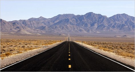
Fig 1: Input Image to study layers

2.1 Absolute Value Layer

• See “absValLayer_example.prototxt”.
• The type is “absVal”. • Function: y = m o d (x ), where, m o d ( ), represents modulus function.
• Input to the layer: NxCxHxW sized blob
• Output from the layer: NxCxHxW sized blob. Fig 2. is an image with three channel outputs after passing from this layer

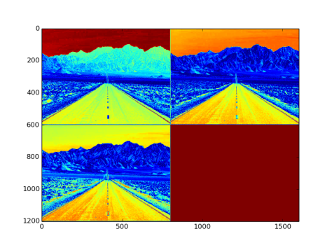
Fig 2: 3 channel output after being passed through absVal layer

2.2 Accuracy Layer

• see “accuracyLayer_example.prototxt”.
• type : “Accuracy”
• Usage: After the final layer. It is used in the TEST phase.
• Takes input as the final layers output and the labels.
• Used for calculating the accuracy of the training during TEST phases.

2.3 ArgMax Layer

• see “argMaxLayer_example.prototxt”
• type: “ArgMax”
• Calculates index of k maximum values across all dimensions
• Usage: After classification layer to get the top-k predictions
• Parameters:
  • top_k: sets the value of k
  • out_max_val: true/false ( if true returns pair (max_index, max_value) the input)
• Fig3. Shows how the output looks, (doesn’t makes sense to get a figure out of the max_values, but still)

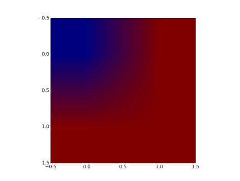
Fig 3: Output after being passed through argMax layer

2.4 Batch Normalization layer

• see “batchNormLayer_example.prototxt”
• Normalizes the input data to achieve mean = 0 and variance = 1.
• Input to the layer: NxCxHxW sized blob
• Output from the layer: NxCxHxW sized blob. Fig 4. is an image with three channel outputs after passing from this layer

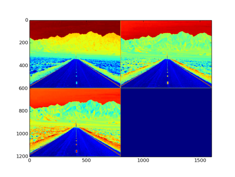
Fig 4: Output after batch normalization

2. 5 Batch Reindex layer

• type: BatchReindex
• To select, reorder, replicate batches

2.6 BNLL Layer

• see “bnllLayer_example.prototxt”
• type: “BNLL”
• bnll: Binomial normal log likelihood [ BNLL ] • Function: y = x + lo g (1 + e x p ( – x )) , if x>0

y = l o g (1 + e x p (x )); if x<=0

• Input to the layer: NxCxHxW sized blob
• Output from the layer: NxCxHxW sized blob. Fig 5. is an image with three channel outputs after passing from this layer

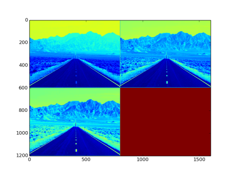
Fig 5: Output after passing through bnll layer

2.7 Concat Layer

• type: “Concat”
• Used to concatenate set of blobs to one blob
• Input: K inputs of dimensions NxCxHxW
• Output: if parameter:
  • axis = 0: Dimension : (K*N)xCxHxW
  • axis = 1: Dimension : Nx(K*C)xHxW

2.8 Convolution Layer

• The most important layer
• see “convLayer_example.prototxt”
• param{} : Its for learning rate and decay rate for filters and biases. First call is for learning rate, next call is for biases. That is why it is written two times.
  • lr_mult: For learning rate
  • decay_mult: Decay rate for the layer Note: This is common to many layers
• type: “Convolution”
• Parameters:
  • num_output(N) : number of filters to be used
  • kernel_size(F): Size of the filter. This can also be mentioned as:
    • kernel_w(F_W)
    • kernel_h(F_H)
  • stride(S): Decides by how much pixel should the filter move over a particular blob in blob dimensions. This is the main reason for sparsity in CNNs. This can also be mentioned as:
    • stride_w(S_W)
    • stride_h(S_H)
  • pad(P): Mentions the size of ZERO padding to be put outside the boundary of the blob. This can also be mentioned as:
    • pad_w(P_W)
    • pad_h(P_H)
  • dilation: Default->1. For morphological operations
  • group: see [ http://colah.github.io/posts/2014-12-Groups-Convolution/%5D
  • bias_term: For adding biases
  • weight_filler: Will be discussed in later sections
  • Input: Blob size of NxCxHxW
  • Output Blob size of N’xC’xH’xW’
    • N’ = N
    • C’ = K
    • W’ = ((W  – F_W + 2 * (P_W ))/S_W ) + 1
    • H’  = ((H  – F_H + 2 * (P_H ))/ S_H ) + 1
  • Fig 6 shows the filters initialized with guassian distribution, and Fig 7 shows the convoluted outputs. ( Note: The actual dimensions of filters/blobs are modified to fit in as images)

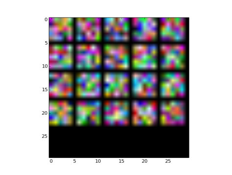
Fig6: Filters initialzed for convolutional layer

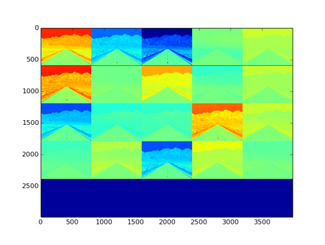
Fig 7: Output blob as images after being passed through convolution layers

2.9 Deconvolution Layer

• see “deconvLayer_example.prototxt”
• Everything same as convolutional layer but, the forward and backward functionalities are reversed.
• Even the parameter functioning is reversed, i.e., pad removes padding, stride causes upsampling, etc.
• Fig 8 shows deconvoluted image blob formed from Fig.7 convoluted images. Exact input image is not restored here because of random weight initialization

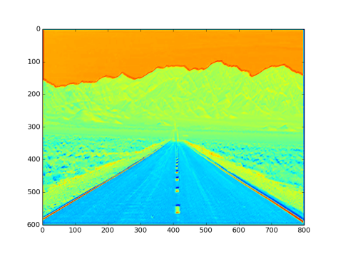
Fig 8: Output after passing through deconvolution layer

Note: This layer can have mutilple channeled output too.

2.10 Dropout Layer

• Note: Works only in TRAIN phase
• see “ dropoutLayer_example.prototxt”
• Function: Sets a portion of pixels to 0, other wise works as absVal Layer.
• Parameters:
  • dropout_ratio: Probability that the current pixel value will be set to zero
• Helps in decreasing the training time.
• Input to the layer: NxCxHxW sized blob
• Output from the layer: NxCxHxW sized blob. Fig 9. is an image with three channel outputs after passing from this layer

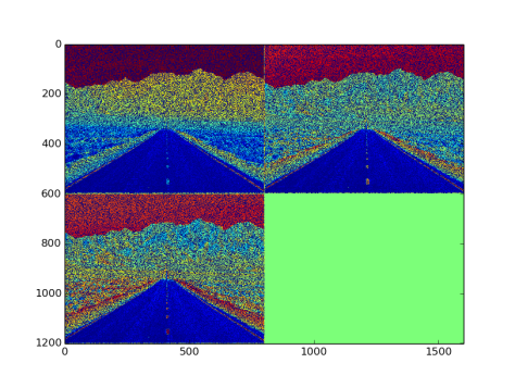
Fig 9: Output after dropout layer

2.11 Element Wise Layer

• type: Eltwise
• For Element wise summation on one or multiple same sized blobs.
• see “eltwiseLayer_example.prototxt”
• Sums up every pixel, basically adds two blobs
• Input to the layer: NxCxHxW sized blob
• Output from the layer: NxCxHxW sized blob. Fig 10. is an image with three channel outputs after passing from this layer

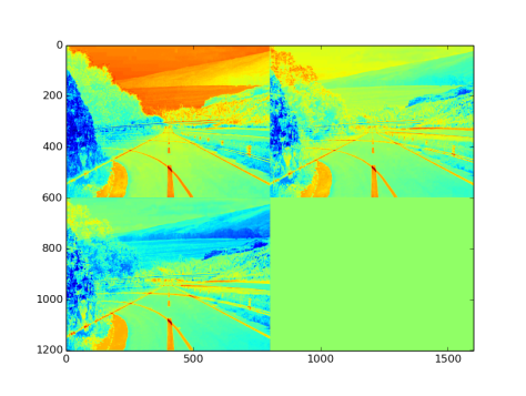
Fig 10: Output after passing through eltwize Layer.

2.12 Embed Layer

• type: Embed
• Same as a fully connected layer, see 2.17
• Except the output blob is a 1D 1-hot vectors. 1-hot vectors are those vectors which have only one element which has value greater than 0, rest all will be zero. [ One Hot Vector ]

2.13 Exponential Layer

• see “expLayer_example.prototxt”
• type: Exp
• Function: y = γ^(α*x + β)
• Parameters:
  • Base (γ) : default: e
  • Scale (α) : default: 1
  • Shift (β) : default: 0
• Input to the layer: NxCxHxW sized blob
• Output from the layer: NxCxHxW sized blob. Fig 11. is an image with three channel outputs after passing from this layer

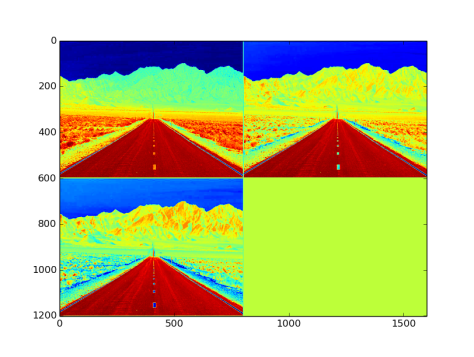
Fig 11: Output from exponential layer with default parameters

2.14 Filter Layer

• type: Filter
• Takes more than one blobs. The last blob is the filter_decision blob. This blob must be a singleton. The selector blob must be of dimensions Nx1x1x1. So whichever element in this blob is 0, the corresponding indexed batch will become 0, and the other ones will be passed as it is.

2.15 Flatten Layer

• type: Flatten
• Takes a blob and flattens its dimensions
• Input dimension: NxCxHxW
• Output dimension: Nx(C*H*W)x1x1

2.16 Image to Col Layer

• type: Im2col
• Used by convolution layer to convert 2D image to a column vector

2.17 Inner Product Layer

• In common terms called as Fully Connected layer
• The next most important layer after convolution layer • see “innerProductLayer.prototxt”
• type: InnerProduct
• Parameter:
  • num_output: Number of neurons in the output layer
  • weight, bias, layer param are same as in convolution layer

2.18 Log Layer

• see “logLayer_example.prototxt”
• type: Log
• Function: 
• Parameters:
  • Base (γ) : default: e
  • Scale (α) : default: 1
  • Shift (β) : default: 0
• Input to the layer: NxCxHxW sized blob
• Output from the layer: NxCxHxW sized blob. Fig 12. is an image with three channel outputs after passing from this layer

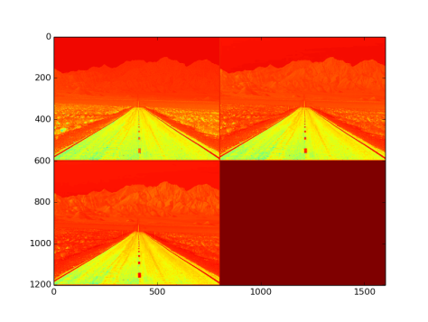
Fig 12: Output from logLayer with default parameters

2.19 LRN Layer

• see “lrnLayer_example.prototxt”
• type: LRN
• LRN: Local response Normalization [ LRN Layer ] [ LRN Function ]
• Parameters
  • local_size: The size of local kernel. Must be an odd number
  • alpha: ideally 0.0001
  • beta: ideally 0.75
  • k: ideally 2
  • norm_region: WITHIN_CHANNEL or ACROSS_CHANNELS (self explanatory)
• Input to the layer: NxCxHxW sized blob
• Output from the layer: NxCxHxW sized blob. Fig 13. is an image with three channel outputs after passing from this layer

Fig 13: Output from lrnLayer with default parameters

2.20 MVN Layer

• See “mvnLayer_example.prototxt”
• type: MVN • MVN: Multi Variate Normalization [ MVN Distribution]
• Parameters:
  • across_channes: bool type
  • normalize_variance: bool type
  • eps: Scalar shift (see link above)
• Input to the layer: NxCxHxW sized blob
• Output from the layer: NxCxHxW sized blob. Fig 14. is an image with three channel outputs after passing from this layer

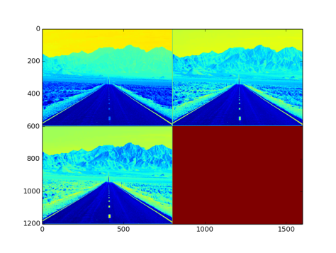
Fig 14: Output after MVN layer

2.21 Pooling Layer

• This is again one of the most frequently used layers in a CNN
• see “poolingLayer_example.prototxt”
• type: Pooling
• Parameters:
  • kernel_size: same as in convolution layer
  • stride: same as in convolution layer
  • pad: same as in convolution layer
  • pool:
    • MAX: Takes max element of the kernel
    • AVE: Takes average of the kernel
    • STOCHASTIC: Not implemented
• Input Dimensions: NxCxHxW
• Output Dimensions: N’xC’xH’xW’ (see 2.8)
  • N’ = N
  • C’ = C
  • W’ = ((W – F_W + 2 * (P_W ))= S_W ) + 1
  • H’  = ((H – F_H + 2 * (P_H ))= S_H ) + 1
• Fig 15. is an image with three channel outputs after passing from this layer

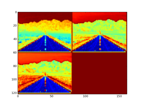
Fig 15: Pooling layer applied with F = 10 and S = 10

2.22 Power Layer

• see “powerLayer_example.prototxt”
• type: Power
• Function: 
• Parameters:
  • Power (γ) : default: 1
  • Scale (α) : default: 1
  • Shift (β) : default: 0
• Input to the layer: NxCxHxW sized blob
• Output from the layer: NxCxHxW sized blob. Fig 16. is an image with three channel outputs after passing from this layer

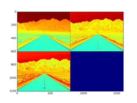
Fig 16: Output after passing through power layer with power = 2, scale = 1, and shift = 2

2.23: PReLU Layer

• The rectified activation function most commonly used as it does not saturate like sigmoid and is even faster. This is prefered over simple ReLU for the fact that it considers the negative input also. [ https://en.wikipedia.org/wiki/Rectifier_ (neural_networks) ]
• see “preluLayer_example.prototxt”
• type: PReLU
• Function: y = m a x ( 0, x ) + α * m in (0, x ), the slope parameter α is constant
• Parameters:
  • channel_shared: bool type (Same alpha for all the channels)
  • filler(will be discussed in later sections)
• Input to the layer: NxCxHxW sized blob
• Output from the layer: NxCxHxW sized blob. Fig 17. is an image with three channel outputs after passing from this layer

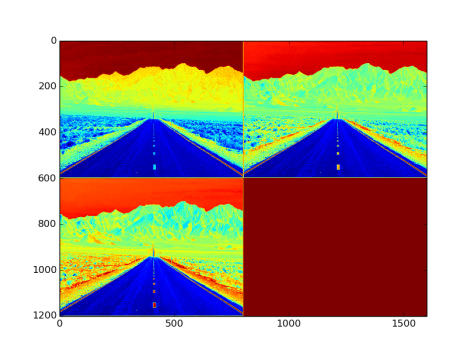
Fig 17: Output after PReLU layer with channels shared and gaussian type filler

2.24 ReLU Layer

• Rectified Linear Units
• PReLU with slope parameter α as non-constant, as in specified by user
• see “reluLayer_example.prototxt”
• type: ReLU
• function: y = m a x ( 0 , x ) + α * m in (0 , x )
• Parameters:
  • negative_slope: Default: 0
• Input to the layer: NxCxHxW sized blob
• Output from the layer: NxCxHxW sized blob. Fig 18. is an image with three channel outputs after passing from this layer .

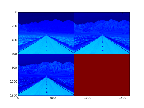
Fig 18: Output after ReLU layer with a negative image input

2.25 Sigmoid Layer

• see “sigmoidLayer_example.prototxt”
• type: Sigmoid
• Used as an activation function
• Function : 
• Input to the layer: NxCxHxW sized blob
• Output from the layer: NxCxHxW sized blob. Fig 19. is an image with three channel outputs after passing from this layer

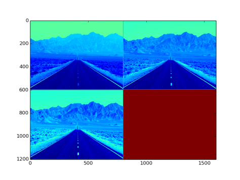
Fig 19: Output after Sigmoid Layer

2.26 Softmax Layer

• see “softmaxLayer_example.prototxt”
• type: Softmax
• Function: [ source: Softmax Layer ]
• Parameters:
  • axis: the central axis (integer type)
• Input to the layer: NxCxHxW sized blob
• Output from the layer: NxCxHxW sized blob. Fig 20. is an image with three channel outputs after passing from this layer

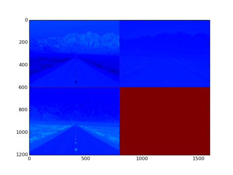
Fig 20: Output after Softmax Layer

2.27 Split Layer

• type: Split
• Creates multiple copies of the input to be fed into different layers ahead simultaneously

2.28 Spatial Pyramid Pooling : Will Update this soon

2.29 TanH Layer

• see “tanhLayer_example.prototxt”
• type: TanH
• Function : 
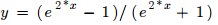
• Input to the layer: NxCxHxW sized blob
• Output from the layer: NxCxHxW sized blob. Fig 21. is an image with three channel outputs after passing from this layer

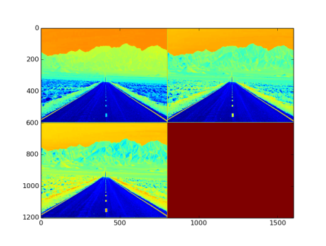
Fig 21: Output after passing tanH layer

 

3. Weight Initializers

They are important because of the fact that initializing weights at complete random may lead to early saturation of the weights. In the examples below, layer used is convolutional layer.

3.1 Constant Filler

• See “constantFiller_example.prototxt”
• type: constant
• Fills the weights with a particular constant, default value is 0
• Parameters
  • value: double type
• Fig 22 and Fig 23 show the filters and effects respectively

Fig 22: Constant fillers of value 0.5

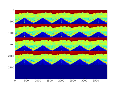
Fig 23: Effect on image by constant type filler and convolutional layer

3.2 Uniform Layer

• see “uniformFiller_example.prototxt”
• type: uniform
• Fills with uniform values between specofied minimum and maximum limits
• Parameters:
  • min: Minimum limit, double type
  • max: Maximum limit, double type
• Fig 24 and Fig 25 show the filters and effects respectively

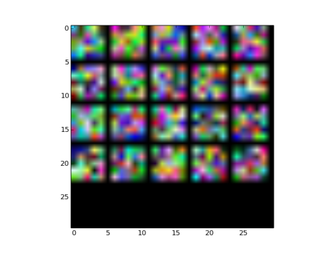
Fig 24: Unifrom filler filters with bundary [0.0, 1.0]

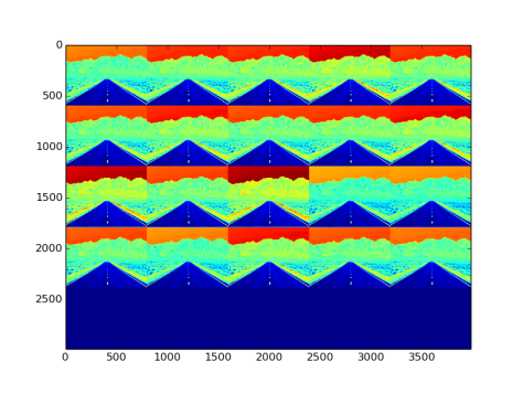
Fig 25: Effect on image by uniform type filler and convolutional layer

3.3 Gaussian Filler

• see “gaussianFiller_example.prototxt”
• type: gaussian [ Gaussian Distribution ]
• Fills data with gaussian distributed values
• Parameters:
  • mean: Double value
  • sparse: Specifies sparseness over the filler. 0 <= sparse <= num_of_outputs (conv layer), integer type [ http://arxiv.org/abs/1402.1389 ]
• Fig 26 and Fig 27 show the filters and effects respectively

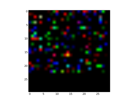
Fig 26: Gaussian filler type Filters with mean = 0.5 and sparse = 3

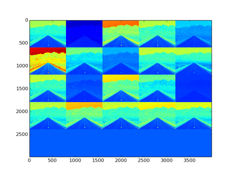
Fig 27: Effect on image by gaussian type filler filters and convolutional layer

3.4 Positive Unit Ball Filler

• see “positiveunitballFiller_example.prototxt”
• type: positive_unitball
• Unit ball: Positive values of an unit sphere centered at zero[ Unit Sphere ] [Unit Ball ]
• Fig 28 and Fig 29 show the filters and effects respectively

Fig 28: Positive unit ball type fillers, note that the image is not blank, the values are very small to be clearly visible over a rgb space

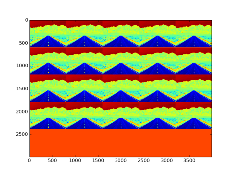
Fig 29: Effect on image by positive unit ball type filler filters and convolutional layer

3.5 Xavier Filler

• see “xavierFiller_example.prototxt”
• type: xavier
• Fills with uniform distribution over the boundary (-scale, scale).
  • scale = sqrt(3/n), where
    • n = FAN_IN(default) = C*H*W, or
    • n = FAN_OUT = N*H*W, or
    • n = (FAN_IN + FAN_OUT)/2
• Parameters:
  • variance_norm: FAN_IN or FAN_OUT or AVERAGE
• Fig 30 and Fig 31 show the filters and effects respectively

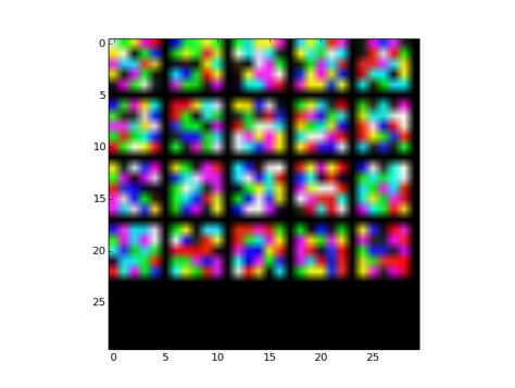
Fig 30: Xavier filler type Filters with default parameters

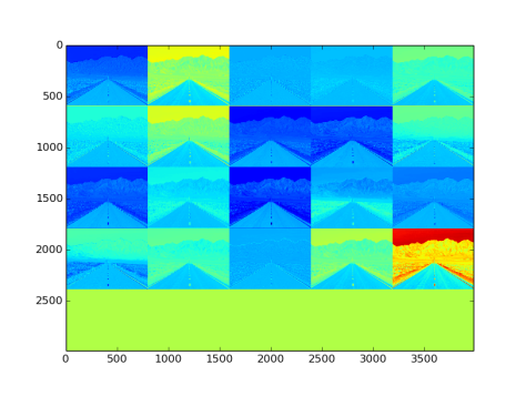
Fig 31: Effect on image by xavier type filler filters and convolutional layer

3.6 MSRA Filler

• see “msraFiller_example.prototxt”
• type: msra
• Fills with ~N(0,variance) distribution.
• variance is inversely proportional to n , where
  • n = FAN_IN(default) = C*H*W, or
  • n = FAN_OUT = N*H*W, or
  • n = (FAN_IN + FAN_OUT)/2
• Parameters:
  • variance_norm: FAN_IN or FAN_OUT or AVERAGE
• Fig 32 and Fig 33 show the filters and effects respectively

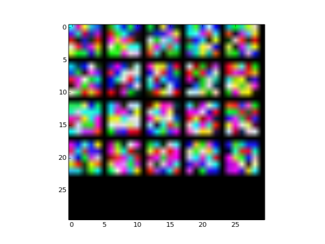
Fig 32: MSRA filler initialized filters

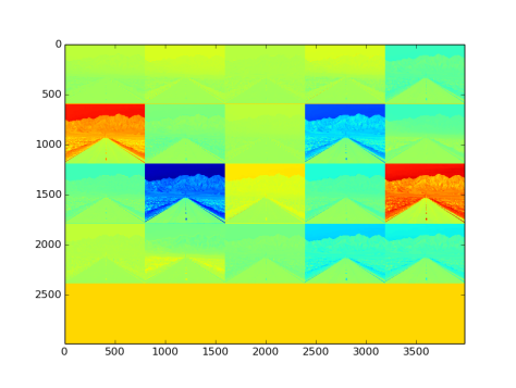
Fig 33: Effect on image by msra type filler filters and convolutional layer

3.7 Bilinear Filler

• see “bilinearFiller_example.prototxt”
• type: bilinear
• Commonly used with deconvolution layer
• Fills the weights with bilinear map function (coefficients of bilinear map interpolation function [ Bilinear Function] [ Bilinear Interpolation]
• Fig 34 and Fig 35 show the filters and effects respectively

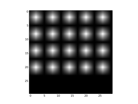
Fig 34: Biliear filler type initialted filters

Fig 35: Effect on image by bilinear type filler filters and convolutional layer

4. Loss Functions

The loss functions enables to find the norm distance between the expected output and the actual output. This section contains a few examples which make use of solvers which are discussed in the next section.

Pre-requisites for this layer:

• Image Dataset: Using Mnist Images.
  • See Section 1 • Annotations: Train.txt
• Annotations: Train.txt and Test.txt
  • These files contain lines in the format /path/to/image/image_name.ext label
  • Please note that the Test.txt points to test dataset which is used for validation during training
• Training net: {will change with all the sub-sections below}
  • This file format is as written in the sequence given below
  • Network name
  • Data layer (both with TRAIN and TEST phases
  • All the layers in the network one after the other
  • Accuracy and Loss layers
• Solver Properties: basic_conv_solver.prototxt
  • See section 5 (To make things more clearer)
• Training initiater: train_net.py
  • All import libraries same as in understandLayers.py
  • Commented enough for self understanding.

4.1 Softmax Layer

• see “softmaxwithlossLayer_example.prototxt”
• type: SoftmaxWithLoss [ Softmax Regression ]
• Inputs:
  • NxCxHxW blob. Values can be (-infinite, infinite )
  • Nx1x1x1 integer label blob
• Outputs:
  • 1x1x1x1 double type output blob
  • Eg output after running the training (copied from terminal):
    • I0204 16:18:08.740026 24219 solver.cpp:237] Iteration 0, loss = 2.30319
• Parameters:
  • ignore_label: To ignore a particular label while calculating the loss.
  • normalize: Bool value (0/1) Normalizes output
  • normalization:
    • FULL
    • VALID
    • BATCH_SIZE

4.2 Hinge Loss Layer

• see “hingelossLayer_example.prototxt”
• type: HingeLoss [ Hinge Loss ]
• Mainly used for one-of-many classification tasks [ Muticlass Classification ]
• Inputs:
  • NxCxHxW blob. Values can be (-infinite, infinite)
  • Nx1x1x1 integer label blob
• Outputs:
  • 1x1x1x1 double type output blob
  • Eg output after running the training (copied from terminal):
    • I0204 16:53:15.270072 25208 solver.cpp:237] Iteration 0, loss = 10.1329
• Parameters:
  • ignore_label: To ignore a particular label while calculating the loss.
  • normalize: Bool value (0/1) Normalizes output
  • normalization:
    • FULL
    • VALID
    • BATCH_SIZE
  • norm:
    • L1
    • L2

4.3 Contrastive Loss 

• type: ContrastiveLoss [ Contrastive loss ] [ Siamese Network ]
• Used to train Siamese Network

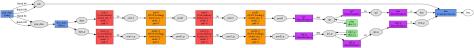
Fig 36: Siamese Network from caffe examples

• Always put after Inner Product layer
• Inputs:
  • NxCx1x1, feature blob a, Values can be (-infinite, infinite)
  • NxCx1x1, feature blob b, Values can be (-infinite, infinite)
  • Nx1x1x1, binary similarity.
• Outputs:
  • 1x1x1x1 double type output blob

4.4 Euclidean Loss Layer

• type: EuclideanLoss [ Euclidean Loss ]
• Basically L2 Norm function over a 4D blob
• Used for real value regression tasks
• Inputs:
  • NxCxHxW blob. Values can be (-infinite, infinite)
  • NxCxHxW target blob. Values can be (-infinite, infinite)
  •  Outputs:
    • 1x1x1x1 double type output blob
• Parameters: None

4.5 Infogain Loss Layer

• type: InfogainLoss [ Infogain Lossf ]
• Its a variant of Multinomial logistic loss function
• Inputs:
  • NxCxHxW blob. Values can be [0,1]
  • Nx1x1x1 integer label blob
  • (Optional) 1x1xKxK Infogain matrix, where k = C*H*W
• Outputs:
  • 1x1x1x1 double type output blob

4.6 Multinomial Logistic Loss Layer

• type: MultinomialLogisticLoss [ Multinomial Logistic Regression]
• Used in cases of one-of-many classification
• Inputs:
  • NxCxHxW blob. Values can be [0,1]
  • Nx1x1x1 labels. Values can be integer
• Outputs:
  • 1x1x1x1 double type output blob
• Parameters: None

4.7 Sigmoid Cross Entropy Layer

• type: SigmoidCrossEntropyLoss [ Cross Entropy ]
• Used in cases of one-of-many classification
• Inputs
  • NxCxHxW blob. Values can be (-infinite, infinite)
  • NxCxHxW target blob. Values can be [0,1]
  • Outputs:
    • 1x1x1x1 double type output blob
• Parameters: None

5. Solvers

These are essential to back-propagate errors in case of supervised learning as they handle very crucial network parameters. Before Diving into the type of solvers this section mentions the basic properties of a solver.

The solver properties are stored in a “prototxt” file

• see “solver_example.prototxt”
• average_loss: double type, must be non-negative
• random_seed: for generating set of random values to be used wherever called in training/testing
• train_net:
  • Must contain the filename of training net prototxt file.
  • String type
  • Must be called only once
  • Other alternatives: net, net_param, train_net_param
• test_iter:
  • While in the test phase, how many iterations it must go through to get the average test results
  • int type
• test_interval:
  • Specifies after how many training iterations, the TEST phase should be placed in.
  • int type
• test_net:
  • Usually the train net itself
  • In the train net, while writing the data layer, this TEST phase is defines, see section 1.
• display:
  • Display details after the specified number of iterations
  • int type
• debug_info:
  • bool type (0/1)
  • Personally recommend to keep this high to understand the network, Note: training time increases due to printing of details
• snapshot:
  • Save snapshots after every specified number of iterations
  • int type
• test_compute_loss:
  • bool type (0/1)
  • Computes loss and displays it on terminal in test phase
  • Personally recommend to keep this high to understand the network, Note: training time increases due to printing of details
• snapshot_format:
  • BINARYPROTO
  • HDF5
  • If not mentioned, stores as .caffemodel
• snapshot_prefix:
  • String type
  • Usually a snapshot is saved as for example “_iter_1.caffemodel”. This specified value here acts as a prefix to that.
  • Helpful if model storage location is not the Parent Directory
• max_iter:
  • int type
  • Specifies the maximum number of iterations the network may have.

Note All the solvers in caffe are derived from Stochastic Gradient Descent Solver

5.1 SGD Solver

• Stochastic Gradient Descent Solver : Like gradient descent but only difference is that by using this the network makes sure that it does not go through every possible training image to update the weights, but goes through only a batch of images, i.e., the stochastic property.
  • Note: All the parameters will be specified in the “solver.prototxt” file
  • Note: By Sub_Parameters it is meant that when you chose a particular lr_policy, the correponding Sub_Parameters must also be mentioned in the solver.prototxt
• Parameters
  • type: “SGD”
  • lr_policy [ Learning Rate ] [ Learning Rate Policy]:
    • String type
    • Defines the learning rate policy
    • Types of lr_policy:
      • “fixed”
        • Sub_Parameters:
          • base_lr:
            • double type
            • Gives the initial system learning rate
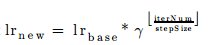
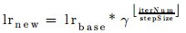
      • “step”
        • function: 
        • Sub_Parameters:
          • base_lr:
            • double type
            • Gives the initial system learning rate
          • gamma:
            • double type
            • Decay rate
          • stepsize:
            • int type
            • Specifies the step uniform intervals
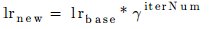
      • “exp”
        • function: 
        • Sub_parameters:
          • base_lr:
            • double type
            • Gives the initial system learning rate
          • gamma:
            • double type
            • Decay rate
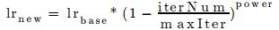
      •  “inv”
        • function: 
        • Sub_parameters:
          • base_lr:
            • double type
            • Gives the initial system learning rate
          • gamma:
            • double type
            • Decay rate
          • power:
            • double type
      • “multistep”
        • function: 
        • Sub_Parameters:
          • base_lr:
            • double type
            • Gives the initial system learning rate
          • gamma:
            • double type
            • Decay rate
          • stepvalue_size:
            • int type
            • Specifies the max step size
        • Like “step”, but has variable step
      • “poly”
        • function: 
        • Sub_parameters:
          • base_lr:
            • double type
            • Gives the initial system learning rate
          • power:
            • double type
      • “sigmoid”
        • function: 
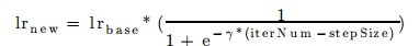
        • Sub_parameters:
          • base_lr:
            • double type
            • Gives the initial system learning rate
          • gamma:
            • double type
            • Decay rate
          • stepsize:
            • int type
            • Specifies the step uniform intervals
  • clip_gradients:
    • Double type
    • if the L2 loss difference obtained is greater than this, then gradients are scaled down by a factor of clipGradients/L2 Loss Difference
  • weight_decay:
    • Double type
    • How is it different from learning rate? [ Decay Rate and Learning Rate] [ Weight Decay ]
      • Sub_Parameters:
        • regularization_type:
          • String type
          • Either “L2“ or “L1“ [ L1 and L2 Losses]
  • momentum:
    • Double type
    • It is a way of pushing the objkective function more quickly along the gradient [ Momentum ] [ Momentum in CNN]
    • It functions in a way that it keeps in mind the details of previous update of weights and uses that to calculate the next step
      • For eg, change in weights v(t) = α * v(t-1) – lr*DifferentialLoss
        • α is the momentum

5.2 AdaDelta Solver

• see [ Ada Delta Optimizer ]
• type: “AdaDelta
• Solver specific parameters:
  • delta: Double type

5.3 AdaGrad Solver

• see [ Ada Grad Optimizer]
• type: “AdaGrad”
• Solver specific parameters:
  • delta: Double type

5.4 RMSProp Solver

• see [ RMSProp Solver]
• type: “RMSProp”
• Solver specific parameters:
  • delta: Double type
  • rms_decay: Double type

5.5 Adam Solver

• see [ http://arxiv.org/abs/1412.6980 ]
• type: “Adam”
• Solver specific parameters:
  • delta: Double type
  • momentum: Double type
  • momentum2: Double type

5.6 Nesterov Solver

• see [ Nesterov Optimisation]
• type: “Nesterov”

 

6. Example LeNet Training using Caffe

6.1 Directory Structure

• Parent Directory
  • Dataset dir
    • Train dir
    • Test dir
  • Train.txt
  • Test.txt
  • lenet_train.prototxt
  • lenet_deploy.prototxt
  • lenet_solver.prototxt
  • lenet_train.py
  • lenet_classify.py
  • lenet_netStats.py
  • lenet_drawNet.py
  • lenet_readCaffeModelFile.py
  • lenet_visualizeFilters.py

Note: Every python file is commented enough to understand the working

6.2 Draw the networks

• run in terminal: sudo ipython lenet_drawNet.py
• see Fig 37 and Fig 38

Fig 37: Deploy Net

Fig 38: Train Net

6.3 Get the blob dimensions and layer dimensions

• run in terminal: sudo ipython lenet_netStats.py
• For blob dimensions the output would be:

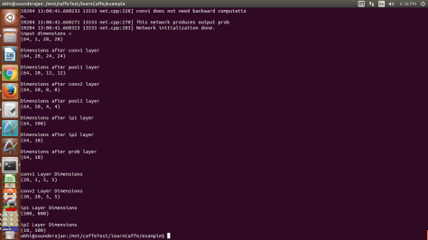
Fig 39: NetStats

6.4 Do training

• run in terminal: sudo ipython lenet_train.py
• End output in the terminal would be:
  • I0204 12:48:38.565213 11798 solver.cpp:326] Optimization Done.
• caffemodel files would be saved in the same folder, it contains trained weights

6.5 Converting snapshots.caffemodel to .txt files

• run in terminal: sudo python lenet_readCaffeModel.py
• It will create a txt file version of the weights

6.6 Lets classify an image now

• run in terminal: sudo python lenet_classify.py
• Sample input image: 
• Classified output:
  • I0205 00:41:10.332895 13227 net.cpp:283] Network initialization done.
  • I0205 00:41:10.337976 13227 net.cpp:816] Ignoring source layer mnist
  • I0205 00:41:10.338515 13227 net.cpp:816] Ignoring source layer loss • Predicted label: 2

That was tough to be classified as 2, but the model did it 🙂 !!!!

6.7 Visualize the layers

• In terminal run : sudo ipython lenet_visualizeFilters.py
• Respective filter and blob images will be generated.

 

This completes the tutorial. If you have any doubts on this please feel free to get back here or on my mail at abhishek4273@gmail.com

Happy Deep Learning 🙂